“My first relationship to any kind of musical situation is
as a listener.”
– Pat Metheny
Music listening [68] is concerned with the understanding of how humans perceive music. As modelers, our goal is to implement algorithms known as machine listening, capable of mimicking this process. There are three major machine-listening approaches: the physiological approach, which attempts to model the neurophysical mechanisms of the hearing system; the psychoacoustic approach, rather interested in modeling the effect of the physiology on perception; and the statistical approach, which models mathematically the reaction of a sound input to specific outputs. For practical reasons, this chapter presents a psychoacoustic approach to music listening.
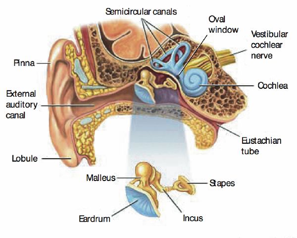
The hearing system is physiologically limited. The torso, head, and outer ear filter the sound field (mostly below 1500 Hz) through shadowing and reflection. The outer ear canal is about 2-cm long, which corresponds to a quarter of the wavelength of frequencies near 4000 Hz, and emphasizes the ear sensitivity to those frequencies. The middle ear is a transducer that converts oscillations in the air into oscillations in the inner ear, which contains fluids. To avoid large losses of energy through reflection, impedance matching is achieved by a mechanical lever system—eardrum, malleus, incus, stapes, and oval window, as in Figure 3-1—that reaches an almost perfect match around 1000 Hz.
Along the basilar membrane, there are roughly 3000 inner hair cells arranged in a regular geometric pattern. Their vibration causes ionic flows that lead to the “firing” of short-duration electrical pulses (the language of the brain) in the nerve fibers connected to them . The entire flow of information runs from the inner ear through approximately 30,000 afferent nerve fibers to reach the midbrain, thalamus, and finally the temporal lobe of the cerebral cortex where is is finally perceived as sound. The nature of the central auditory processing is, however, still very much unclear, which mainly motivates the following psychophysical approach [183].
|
|
Psychoacoustics is the study of the subjective human perception of sounds. It connects the physical world of sound vibrations in the air to the perceptual world of things we actually hear when we listen to sounds. It is not directly concerned with the physiology of the hearing system as discussed earlier, but rather with its effect on listening perception. This is found to be the most practical and robust approach to an application-driven work. This chapter is about modeling our perception of music through psychoacoustics. Our model is causal, meaning that it does not require knowledge about the future, and can be implemented both in real time, and faster than real time. A good review of reasons that motivate and inspire this approach can also be found in [142].
Let us begin with a monophonic audio signal of arbitrary length and sound quality. Since we are only concerned with the human appreciation of music, the signal may have been formerly compressed, filtered, or resampled. The music can be of any kind: we have tested our system with excerpts taken from jazz, classical, funk, electronic, rock, pop, folk and traditional music, as well as speech, environmental sounds, and drum loops.
The goal of our auditory spectrogram is to convert the time-domain waveform into a reduced, yet perceptually meaningful, time-frequency representation. We seek to remove the information that is the least critical to our hearing sensation while retaining the most important parts, therefore reducing signal complexity without perceptual loss. The MPEG1 audio layer 3 (MP3) codec [18] is a good example of an application that exploits this principle for compression purposes. Our primary interest here is understanding our perception of the signal rather than resynthesizing it, therefore the reduction process is sometimes simplified, but also extended and fully parametric in comparison with usual perceptual audio coders.
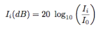
First, we apply a standard Short-Time Fourier Transform (STFT) to obtain a standard spectrogram. We experimented with many window types and sizes, which did not have a significant impact on the final results. However, since we are mostly concerned with timing accuracy, we favor short windows (e.g., 12-ms Hanning), which we compute every 3–6 ms (i.e., every 128–256 samples at 44.1 KHz). The Fast Fourier Transform (FFT) is zero-padded up to 46 ms to gain additional interpolated frequency bins. We calculate the power spectrum and scale its amplitude axis to decibels (dB SPL, a measure of sound pressure level) as in the following equation:
| (3.1) |
where i > 0 is an index of the power-spectrum bin of intensity I, and I0 is an arbitrary threshold of hearing intensity. For a reasonable tradeoff between dynamic range and resolution, we choose I0 = 60, and we clip sound pressure levels below -60 dB. The threshold of hearing is in fact frequency-dependent and is a consequence of the outer and middle ear response.
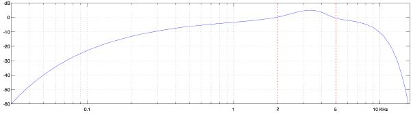
As described earlier, physiologically the outer and middle ear have a great implication on the overall frequency response of the ear. A transfer function was proposed by Terhardt in [160], and is defined in decibels as follows:
|
| (3.2) |
As depicted in Figure 3-2, the function is mainly characterized by an attenuation in the lower and higher registers of the spectrum, and an emphasis around 2–5 KHz, interestingly where much of the speech information is carried [136].
|
|
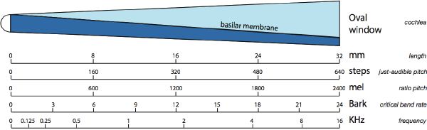
The inner ear (cochlea) is shaped like a 32 mm long snail and is filled with two different fluids separated by the basilar membrane. The oscillation of the oval window takes the form of a traveling wave which moves along the basilar membrane. The mechanical properties of the cochlea (wide and stiff at the base, narrower and much less stiff at the tip) act as a cochlear filterbank: a roughly logarithmic decrease in bandwidth (i.e., constant-Q on a logarithmic scale) as we move linearly away from the cochlear opening (the oval window).
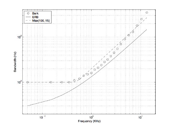
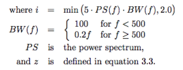
The difference in frequency between two pure tones by which the sensation of “roughness” disappears and the tones sound smooth is known as the critical band. It was found that at low frequencies, critical bands show an almost constant width of about 100 Hz, while at frequencies above 500 Hz, their bandwidth is about 20% of the center frequency. A Bark unit was defined and led to the so-called critical-band rate scale. The spectrum frequency f is warped to the Bark scale z(f) as in equation (3.3) [183]. An Equivalent Rectangular Bandwidth (ERB) scale was later introduced by Moore and is shown in comparison with the Bark scale in figure 3-4 [116].
|
| (3.3) |
|
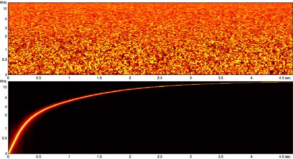
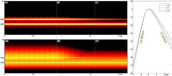
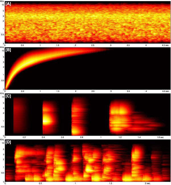
The effect of warping the power spectrum to the Bark scale is shown in Figure 3-5 for white noise, and for a pure tone sweeping linearly from 20 to 20K Hz. Note the non-linear auditory distortion of the frequency (vertical) axis.
Simultaneous masking is a property of the human auditory system where certain maskee sounds disappear in the presence of so-called masker sounds. Masking in the frequency domain not only occurs within critical bands, but also spreads to neighboring bands. Its simplest approximation is a triangular function with slopes +25 dB/Bark and -10 dB/Bark (Figure 3-6), where the lower frequencies have a stronger masking influence on higher frequencies than vice versa [146]. A more refined model is highly non-linear and depends on both frequency and amplitude. Masking is the most powerful characteristic of modern lossy coders: more details can be found in [17]. A non-linear spreading function as found in [127] and modified by Lincoln in [104] is:
|
| (3.4) |
|
(3.5) |
Instantaneous masking was essentially defined through experimentation with pure tones and narrow-band noises [50][49]. Integrating spreading functions in the case of complex tones is not very well understood. To simplify, we compute the full spectral mask through series of individual partials.
|
|
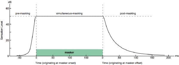
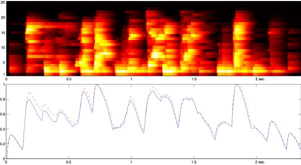
Another perceptual phenomenon that we consider as well is temporal masking. As illustrated in Figure 3-7, there are two types of temporal masking besides simultaneous masking: pre-masking and post-masking. Pre-masking is quite unexpected and not yet conclusively researched, but studies with noise bursts revealed that it lasts for about 20 ms [183]. Within that period, sounds softer than the masker are typically not audible. We do not implement it since signal-windowing artifacts have a similar smoothing effect. However, post-masking is a kind of “ringing” phenomenon which lasts for almost 200 ms. We convolve the envelope of each frequency band with a 200-ms half-Hanning (raised cosine) window. This stage induces smoothing of the spectrogram, while preserving attacks. The effect of temporal masking is depicted in Figure 3-8 for various sounds, together with their loudness curve (more on loudness in section 3.2).
|
|
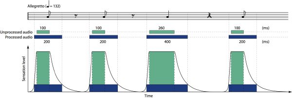
The temporal masking effects have important implications on the perception of rhythm. Figure 3-9 depicts the relationship between subjective and physical duration of sound events. The physical duration of the notes gives an incorrect estimation of the rhythm (in green), while if processed through a psychoacoustic model, the rhythm estimation is correct (in blue), and corresponds to what the performer and audience actually hear.
|
|
Finally, we combine all the preceding pieces together, following that order, and build our hearing model. Its outcome is what we call the audio surface. Its graphical representation, the auditory spectrogram, merely approximates a “what-you-see-is-what-you-hear” type of spectrogram, meaning that the “just visible” in the time-frequency display corresponds to the “just audible” in the underlying sound. Note that we do not understand music yet, but only sound. Figure 3-10 displays the audio surface of white noise, a sweeping pure tone, four distinct sounds, and a real-world musical excerpt.
The area below the audio surface (the zone covered by the mask) is called the excitation level, and minus the area covered by the threshold in quiet, leads to the sensation of loudness: the subjective judgment of the intensity of a sound. It is derived easily from our auditory spectrogram by adding the amplitudes across all frequency bands:
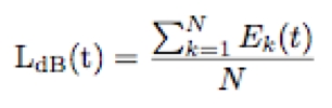
| (3.6) |
where Ek is the amplitude of frequency band k of total N in the auditory spectrogram. Advanced models of loudness by Moore and Glasberg can be found in [117][57]. An example is depicted in Figure 3-11.
Timbre, or “tone color,” is a relatively poorly defined perceptual quality of sound. The American Standards Association (ASA) defines timbre as “that attribute of sensation in terms of which a listener can judge that two sounds having the same loudness and pitch are dissimilar” [5]. In music, timbre is the quality of a musical note that distinguishes musical instruments. It was shown by Grey [66] and Wessel [168] that important timbre characteristics of the orchestral sounds are attack quality (temporal envelope), spectral flux (evolution of the spectral distribution over time), and brightness (spectral centroid).
In fact, this psychoacoustician’s waste basket includes so many factors that the latest trend for characterizing timbre, sounds, and other high-level musical attributes consists of using a battery of so-called low-level audio descriptors (LLD), as specified for instance in the MPEG7 standardization format [118]. Those can be organized in various categories including temporal descriptors computed from the waveform and its envelope, energy descriptors referring to various energy measurements of the signal, spectral descriptors computed from the STFT, harmonic descriptors computed from the sinusoidal harmonic modeling of the signal, and perceptual descriptors computed using a model of the human hearing process [111][133][147].
|
|
The next step typically consists of finding the combination of those LLDs, which hopefully best matches the perceptive target [132]. An original approach by Pachet and Zils substitutes the basic LLDs by primitive operators. Through genetic programming, the Extraction Discovery System (EDS) aims at composing these operators automatically, and discovering signal-processing functions that are “locally optimal” for a given descriptor extraction task [126][182].
Rather than extracting specific high-level musical descriptors, or classifying sounds given a specific “taxonomy” and arbitrary set of LLDs, we aim at representing the timbral space of complex polyphonic signals with a meaningful, yet generic description. Psychoacousticians tell us that the critical band can be thought of as a frequency-selective channel of psychoacoustic processing. For humans, only 25 critical bands cover the full spectrum (via the Bark scale). These can be regarded as a reasonable and perceptually grounded description of the instantaneous timbral envelope. An example of that spectral reduction is given in Figure 3-11 for a rich polyphonic musical excerpt.
Onset detection (or segmentation) is the means by which we can divide the musical signal into smaller units of sound. This section only refers to the most atomic level of segmentation, that is the smallest rhythmic events possibly found in music: individual notes, chords, drum sounds, etc. Organized in time, a sequence of sound segments infers our perception of music. Since we are not concerned with sound source separation, a segment may represent a rich and complex polyphonic sound, usually short. Other kinds of segmentations (e.g., voice, chorus) are specific aggregations of our minimal segments which require source recognition, similarity, or continuity procedures.
Many applications, including the holy-grail transcription task, are primarily concerned with detecting onsets in a musical audio stream. There has been a variety of approaches including finding abrupt changes in the energy envelope [38], in the phase content [10], in pitch trajectories [138], in audio similarities [51], in autoregressive models [78], in spectral frames [62], through a multifeature scheme [162], through ICA and hidden Markov modeling [1], and through neural networks [110]. Klapuri [90] stands out for using psychoacoustic knowledge; this is the solution proposed here as well.
We define a sound segment by its onset and offset boundaries. It is assumed perceptually “meaningful” if its timbre is consistent, i.e., it does not contain any noticeable abrupt changes. Typical segment onsets include abrupt loudness, pitch or timbre variations. All of these events translate naturally into an abrupt spectral variation in the auditory spectrogram.
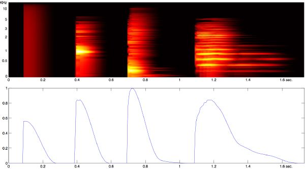
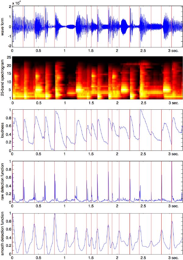
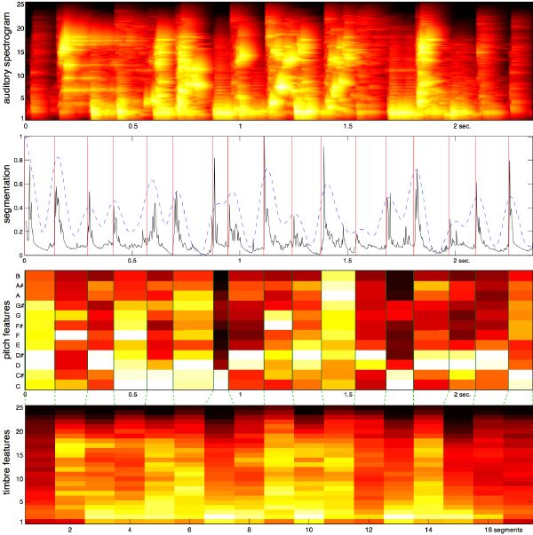
We convert the auditory spectrogram into an event detection function by calculating the first-order difference function of each spectral band, and by summing across channels. The resulting signal reveals peaks that correspond to onset transients (Figure 3-12, pane 4). Transients within a 50-ms window typically fuse perceptually into a single event [155]. We model fusion by convolving the raw event detection signal with a Hanning window. Best results (i.e., with segments greater than 50 ms) are obtained with a 150-ms window. The filtering generates a smooth function now appropriate for the peak-picking stage. Unlike traditional methods that usually rely heavily on designing an adaptive threshold mechanism, we can simply select the local maxima (Figure 3-12, pane 5). We may reject the flattest peaks through threshold as well, but this stage and settings are not critical.
Since we are concerned with reusing the audio segments for synthesis, we refine the onset location by analyzing it in relation with its corresponding loudness function. An onset generally occurs with an increase variation in loudness. To retain the entire attack, we seek the previous local minimum in the loudness signal (in general a small time shift of at most 20 ms), which corresponds to the softest pre-onset moment, that is the best time to cut. Finally, we look within the corresponding waveform, and search for the closest zero-crossing, with an arbitrary but consistent choice of direction (e.g., from negative to positive). This stage is important to ensure signal continuity at synthesis.
Segment sequencing is the reason for musical perception, and the inter-onset interval (IOI) is at the origin of the metrical-structure perception [74]. The tatum, named after jazz pianist “Art Tatum” in [12] can be defined as the lowest regular pulse train that a listener intuitively infers from the timing of perceived musical events: a time quantum. It is roughly equivalent to the time division that most highly coincides with note onsets: an equilibrium between 1) how well a regular grid explains the onsets, and 2) how well the onsets explain the grid.
The tatum is typically computed via a time-varying IOI histogram [64], with an exponentially decaying window for past data, enabling the tracking of accelerandos and ritardandos [148]. The period is found by calculating the greatest common divisor (GCD) integer that best estimates the histogram harmonic structure, or by means of a two-way mismatch error procedure as originally proposed for the estimation of the fundamental frequency in [109], and applied to tatum analysis in [65][67]. Two error functions are computed: one that illustrates how well the grid elements of period candidates explain the peaks of the measured histogram; another one illustrates how well the peaks explain the grid elements. The TWM error function is a linear combination of these two functions. Phase is found in a second stage, for example through circular mean in a grid-to-onset alignment procedure as in [148].
Instead of a discrete IOI histogram, our method is based on a moving autocorrelation computed on the smooth event-detection function as found in section 3.4. The window length is chosen adaptively from the duration of x past segments to ensure rough salience stability in the first-peak estimation of the autocorrelation (e.g., x ≈ 15). The autocorrelation is only partially calculated since we are guaranteed to find a peak in the ±(100∕x)% range around its center. The first peak gives the approximate tatum period. To refine that estimation, and detect the phase, we run a search through a set of templates.
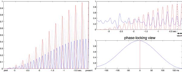
Templates are patterns or filters that we aim to align against the signal. We pre-compute dozens of regular pulse trains in the range 1.5–15 Hz through a series of click trains convolved with a Hanning window: the same used to smooth the detection function in section 3.4.2. To account for memory fading, we shape the templates with a half-raised cosine of several seconds, e.g., 3–6 sec. The templates are finally normalized by their total energy (Figure 3-13, left). At a given estimation time, the optimal template is the one with highest energy when cross-correlated with the current smoothed detection function. For maximum efficiency, we only estimate templates within the range ±10% of our rough period estimation. We limit the cross-correlation lag search for the optimal template, to only the tatum period length Δτ, since it contains the peak that will account for phase offset φ and allows us to predict the next tatum location: τ[i + 1] = τ[i] + Δτ[i] - c ⋅ φ[i] where c is a smoothing coefficient and φ[i] ∈ [-Δτ[i]∕2,+Δτ[i]∕2[. The system quickly phase locks and is efficiently updated at tatum-period rate.
|
|
The beat (or tactus) is a perceptually induced periodic pulse that is best described by the action of “foot-tapping” to the music, and is probably the most studied metrical unit. It defines tempo: a pace reference that typically ranges from 40 to 260 beats per minute (BPM) with a mode roughly around 120 BPM. Tempo is shown to be a useful time-normalization metric of music (section 4.5). The beat is a down-sampled, aligned version of the tatum, although there is no clear and right answer on how many tatum periods make up a beat period: unlike tatum, which is derived directly from the segmentation signal, the beat sensation is cognitively more complex and requires information both from the temporal and the frequency domains.
Beat induction models can be categorized by their general approach: top-down (rule- or knowledge-based), or bottom-up (signal processing). Early techniques usually operate on quantized and symbolic representations of the signal, for instance after an onset detection stage. A set of heuristic and gestalt rules (based on accent, proximity, and grouping) is applied to infer the underlying metrical structure [99][37][159][45]. More recently, the trend has been on signal-processing approaches. The scheme typically starts with a front-end subband analysis of the signal, traditionally using a filter bank [165][141][4] or a discrete Fourier Transform [59][96][91]. Then, a periodicity estimation algorithm—including oscillators [141], histograms [39], autocorrelations [63], or probabilistic methods [95]—finds the rate at which signal events occur in concurrent channels. Finally, an integration procedure combines all channels into the final beat estimation. Goto’s multiple-agent strategy [61] (also used by Dixon [38][39]) combines heuristics and correlation techniques together, including a chord change detector and a drum pattern detector. Klapuri’s Bayesian probabilistic method applied on top of Scheirer’s bank of resonators determines the best metrical hypothesis with constraints on continuity over time [92]. Both approaches stand out for their concern with explaining a hierarchical organization of the meter (section 4.6).
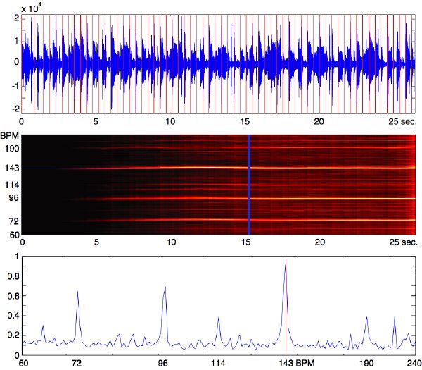
A causal and bottom-up beat tracker based on our front-end auditory spectrogram (25 bands) and Scheirer’s bank of resonators [141] is developed. It assumes no prior knowledge, and includes a confidence value, which accounts for the presence of a beat in the music. The range 60–240 BPM is logarithmically distributed to a large bank of comb filters, whose properties are to resonate at a given tempo. The filters are tested on multiple frequency channels of the auditory spectrogram simultaneously, and are tuned to fade out within seconds, as a way to model short-term memory. At any given time, their internal energy can be summed across channels by tempo class, which results in a tempo spectrum as depicted in Figure 3-14 (bottom). Yet, one of the main drawbacks of the model is its unreliable tempo-peak selection mechanism. A few peaks of the spectrum may give a plausible answer, and choosing the highest is not necessarily the best, or most stable strategy. A template mechanism is used to favor the extraction of the fastest tempo in case of ambiguity1. section 5.3, however, introduces a bias-free method that can overcome this stability issue through top-down feedback control.
Figure 3-14 shows an example of beat tracking a polyphonic jazz-fusion piece at supposedly 143 BPM. A tempogram (middle pane) displays the tempo knowledge gained over the course of the analysis. It starts with no knowledge, but slowly the tempo space emerges. Note in the top pane that beat tracking was stable after merely 1 second. The bottom pane displays the current output of each resonator. The highest peak is our extracted tempo. A peak at the sub octave (72 BPM) is visible, as well as some other harmonics of the beat. A real-time implementation of our beat tracker is available for the Max/MSP environment [180].
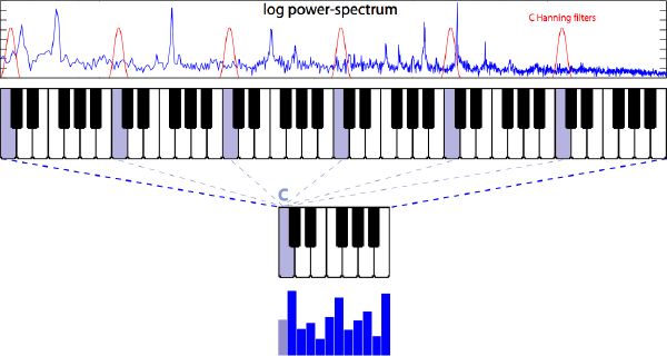
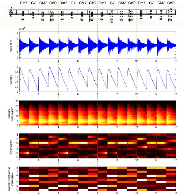
The atomic audio fragments found through sound segmentation in section 3.4 represent individual notes, chords, drum sounds, or anything timbrally and harmonically stable. If segmented properly, there should not be any abrupt variations of pitch within a segment. Therefore it makes sense to analyze its pitch content, regardless of its complexity, i.e., monophonic, polyphonic, noisy. Since polyphonic pitch-tracking is yet to be solved, especially in a mixture of sounds that includes drums, we opt for a simpler, yet quite relevant 12-dimensional chroma (a pitch class regardless of its register) description as in [8]. A chromagram is a representation of chromas against time. It was previously used for chord recognition [178], key analysis [131], chorus detection [60], and thumbnailing [27].
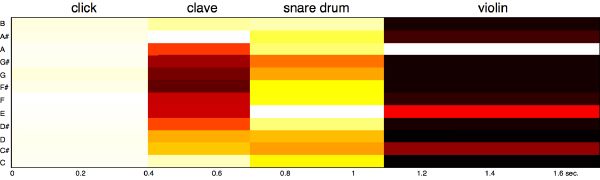
We compute the FFT of the whole segment (generally between 80 to 300 ms long), which gives us sufficient frequency resolution. A standard Hanning window is applied first, which slightly attenuates the effect of noisy transients while emphasizing the sustained part of the segment. A chroma vector is the result of folding the energy distribution of much of the entire power spectrum (6 octaves ranging from C1 = 65 Hz to B7 = 7902 Hz) into 12 discrete pitch classes. This is a fair approximation given that both fundamental and first harmonic correspond to the same pitch class and are often the strongest partials of the sound. The output of the 72 logarithmically spaced Hanning filters of a whole-step bandwidth—accordingly tuned to the equal temperament chromatic scale—is accumulated into their corresponding pitch class (Figure 3-15). The scale is best suited to western music, but applies to other tunings (Indian, Chinese, Arabic, etc.), although it is not as easily interpretable or ideally represented. The final 12-element chroma vector is normalized by dividing each of its elements by the maximum element value. We aim at canceling the effect of loudness across vectors (in time) while preserving the ratio between pitch classes within a vector (in frequency). An example of a segment-synchronized chromagram for four distinct sounds is displayed in Figure 3-16.
|
|
Our implementation differs significantly from others as we compute chromas on a segment basis. The great benefits of doing a segment-synchronous2 computation are:
1. accurate time resolution by short-window analysis of onsets;
2. accurate frequency resolution by adaptive window analysis;
3. computation speed since there is no need to overlap FFTs; and
4. efficient and meaningful representation for future use.
|
|
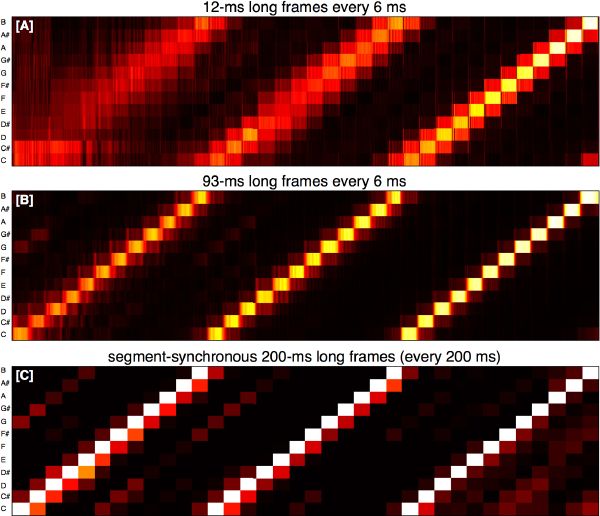
The usual time-frequency paradox and our “simple” solution are shown in Figure 3-17 in the case of a chromatic scale. Our method optimizes both time and frequency analysis while describing the signal in terms of its musical features (onsets and inter-onset harmonic content). Figure 3-18 demonstrates the benefit of our pitch representation in the case of monotimbral music. Indeed, the critical-band representation, suitable for timbre recognition (section 3.3), is not suitable for pitch-content analysis. However, the segment-synchronous chromagram, which discards the timbre effect through its normalization process, appears suitable for describing pitch and harmonic content.
|
|
In this chapter, we have modeled human perception through psychoacoustics. We have constructed a low-level representation of music signals in the form of a sequence of short audio segments, and their associated perceptual content:
1. rhythm represented by a loudness curve3;
2. timbre represented by 25 channels of an auditory spectrogram;
3. pitch represented by a 12-class chroma vector.
Although the pitch content of a given segment is now represented by a compact 12-feature vector, loudness, and more so timbre, are still large—by an order of magnitude, since we still describe them on a frame basis. Empirically, it was found—via resynthesis experiments constrained only by loudness—that for a given segment, the maximum value in the loudness curve is a better approximation of the overall perceived loudness, than the average of the curve. For a more accurate representation, we describe the loudness curve with 5 dynamic features: loudness at onset (dB), maximum loudness (dB), loudness at offset (dB), length of the segment (ms), and time location of the maximum loudness relative to the onset (ms). A currently rough approximation of timbre consists of averaging the Bark features over time, which reduces the timbre space to only 25 Bark features per segment. We finally label our segments with a total of 5 rhythm features + 25 timbral features + 12 pitch features = 42 features4.
Such compact low-rate segment-synchronous feature description is regarded as a musical signature, or signal metadata, and has proven to be efficient and meaningful in a series of applications as demonstrated in chapter 6 . In the following chapter, we interpret this musical metadata through a set of hierarchical structures of pitch, rhythm, and timbre.