“If it sounds good and feels good, then it IS good! ”
– Duke Ellington
The motivation behind this analysis work is primarily music synthesis. We are interested in composing with a database of sound segments—of variable sizes, usually ranging from 60 to 300 ms—which we can extract from a catalog of musical samples and songs (e.g., an MP3 collection). These segments can be rearranged into sequences themselves derived from timbral, harmonic, and rhythmic structures extracted/learned/transformed from existing songs1. Our first application, however, does not rearrange short segments, but rather manipulates entire sections of songs by smoothly transitioning between them.
A DJ (Disc Jockey) is an individual who selects, mixes and plays pre-recorded music for the enjoyment of others. Often, DJs are expected to demonstrate greater technical aspects of their performance by manipulating the songs they play in order to maintain a given tempo and energy level. “Even simply playing records allows for the DJ to bring his own creative ideas to bear upon the pre-recorded music. Playing songs in sequence offers the opportunity to observe relationships forming between different songs. Given careful attention and control, the DJ can create these relations and encourage them to become more expressive, beautiful and telling” [172]. This is called the art of “programming,” or track selection.
Certainly, there is more to the art of DJ-ing than technical abilities. In this first application, however, we are essentially interested in the problem of beat-matching and cross-fading songs as “smoothly” as possible. This is one of DJs most common practices, and it is relatively simple to explain but harder to master. The goal is to select songs with similar tempos, and align their beat over the course of a transition while cross-fading their volumes. The beat markers, as found in section 3.5, are obviously particularly relevant features.
The length of a transition is chosen arbitrarily by the user (or the computer), from no transition to the length of an entire song; or it could be chosen through the detection of salient changes of structural attributes; however, this is not currently implemented. We extend the beat-matching principle to downbeat matching by making sure that downbeats align as well. In our application, the location of a transition is chosen by selecting the most similar rhythmic pattern between the two songs as in section 4.6.3. The analysis may be restricted to finding the best match between specific sections of the songs (e.g., the last 30 seconds of song 1 and the first 30 seconds of song 2).
To ensure perfect match over the course of long transitions, DJs typically adjust the playback speed of the music through specialized mechanisms, such as a “relative-speed” controller on a turntable (specified as a relative positive/negative percentage of the original speed). Digitally, a similar effect is implemented by “sampling-rate conversion” of the audio signal [154]. The procedure, however, distorts the perceptual quality of the music by detuning the whole sound. For correcting this artifact, we implement a time-scaling algorithm that is capable of speeding up or slowing down the music without affecting the pitch.
There are three main classes of audio time-scaling (or time-stretching): 1) the time-domain approach, which involves overlapping and adding small windowed fragments of the waveform; 2) the frequency-domain approach, which is typically accomplished through phase-vocoding [40]; and 3) the signal-modeling approach, which consists of changing the rate of a parametric signal description, including deterministic and stochastic parameters. A review of these methods can be found in [16], and implementations for polyphonic music include [15][94][102][43].
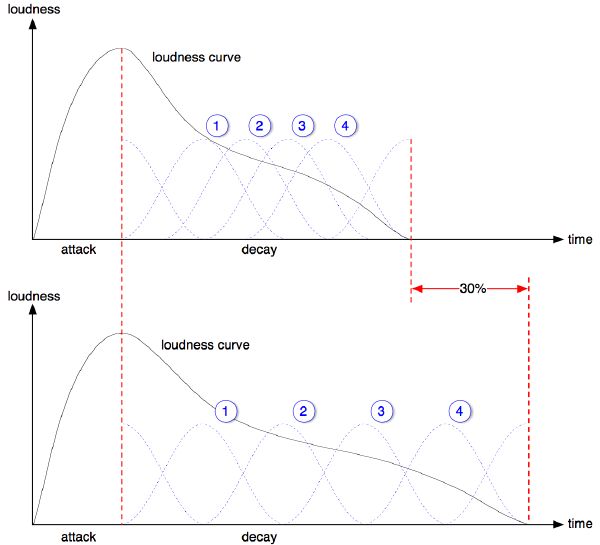
We have experimented with both the time-domain and frequency-domain methods, with certain original properties to them. For instance, it is suggested in [16] to preserve transients unprocessed in order to reduce artifacts, due to the granularity effect of windowing. While the technique has previously been used with the phase vocoder, we apply it to our time-domain algorithm as well. The task is relatively simple since the signal is already segmented, as in section 3.4. For each sound segment, we pre-calculate the amount of required stretch, and we apply a fixed-size overlap-add algorithm onto the decaying part of the sound, as in Figure 6-1. In our frequency implementation, we compute a segment-long FFT to gain maximum frequency resolution (we assume stationary frequency content throughout the segment), and time-scale the strongest partials of the spectrum during decay, using an improved phase-vocoding technique, i.e., by preserving the correlation between phases of adjacent bins for a given partial [97]. Our frequency implementation performs well with harmonic sounds, but does not do well with noisier sounds: we adopt the simple and more consistent time-domain approach.
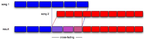
There are several options of cross-fading shape, the most common being linear, exponential, S-type, and constant-power. We choose to implement a constant-power cross-fader in order to preserve the perceptual energy “constant” through the transition. This is implemented with a logarithmic fade curve that starts quickly and then slowly tapers off towards the end (Figure 6-2). In order to avoid clipping when two songs overlap, we implement a simple compression algorithm. Finally, our system adapts continuously to tempo variations by interpolating gradually one tempo into another over the course of a transition, and by time stretching every audio segment appropriately to preserve perfect beat alignment (Figure 6-3). Beat-matching and automatic transitions are successfully accomplished for arbitrary songs where tempos differ by up to 40%. Another interesting variant of the application transitions a song with itself, allowing for extensions of that song to infinity2.
|
|
A sound segment represents the largest unit of continuous timbre, and the shortest fragment of audio in our representation. We believe that every segment could eventually be described and synthesized by analytic methods, such as additive synthesis, but this thesis work is only concerned with the issue of synthesizing music, i.e., the structured juxtaposition of sounds over time. Therefore, we use the sound segments found in existing pieces as primitive blocks for creating new pieces. Several experiments have been implemented to demonstrate the advantages of our segment-based synthesis approach over an indeed more generic, but still ill-defined frame-based approach.
Our synthesis principle is extremely simple: we concatenate (or string together) audio segments as a way to “create” new musical sequences that never existed before. The method is commonly used in speech synthesis where a large database of phones is first tagged with appropriate descriptors (pitch, duration, position in the syllable, etc.). At runtime, the desired target utterance is created by determining the best chain of candidate units from the database. This method, also known as unit selection synthesis, gives the best results in speech synthesis without requiring much signal processing when the database is large enough.
Our concatenation module does not process the audio: there is no segment overlap, windowing, or cross-fading involved, which is typically the case with granular synthesis, in order to avoid discontinuities. Since segmentation is performed psychoacoustically at the most strategic location (i.e., just before an onset, at the locally quietest moment, and at zero-crossing), the transitions are generally artifact-free and seamless.
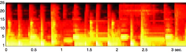
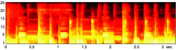
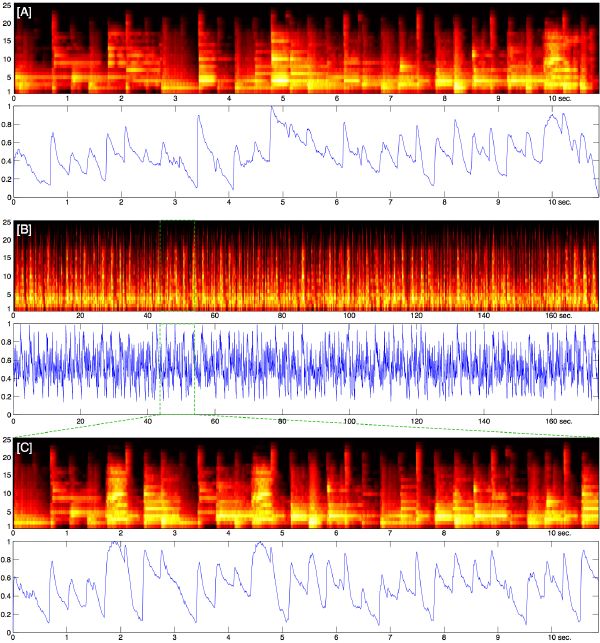
This first of our series of experiments assumes no structure or constraint whatsoever. Our goal is to synthesize an audio stream by randomly juxtaposing short sound segments previously extracted from a given piece of music—about two to eight segments per second with the music tested. During segmentation, a list of pointers to audio samples is created. Scrambling the music consists simply of rearranging the sequence of pointers randomly, and of reconstructing the corresponding waveform. While the new sequencing generates the most unstructured music, and is arguably regarded as the “worst” possible case of music resynthesis, the event-synchronous synthesis sounds robust against audio clicks and glitches (Figure 6-5).
|
|
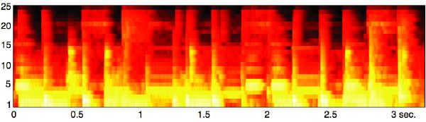
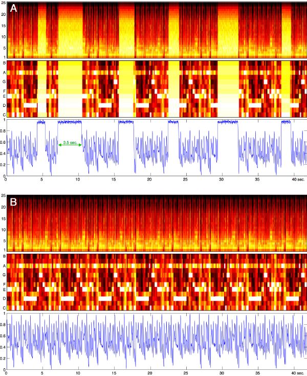
The underlying beat of the music, if it exists, represents a perceptual metric on which segments lie. While beat tracking was found independently of the segment organization, the two representations are intricately interrelated with each other. The same scrambling procedure is applied onto the beat segments (i.e., audio segments separated by two beat markers). As expected, the generated music is metrically structured, i.e., the beat can be extracted again, but the underlying harmonic, and melodic structure are now scrambled.
|
|
The next experiment consists of adding a simple structure to the previous method. This time, rather than scrambling the music, the order of segments is reversed, i.e., the last segment comes first, and the first segment comes last. This is much like what could be expected when playing a score backwards, starting with the last note first, and ending with the first one. This is however very different from reversing the audio signal, which distorts “sounds,” where reversed decays come first and attacks come last (Figure 6-6). Tested on many kinds of music, it was found that perceptual issues with unprocessed concatenative synthesis may occur with overlapped sustained sounds, and long reverb—certain musical discontinuities cannot be avoided without additional processing, but this is left for future work.
|
|
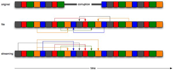
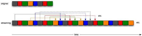
A well-defined synthesis application that derives from our segment concatenation consists of restoring corrupted audio files, and streaming music on the Internet or cellular phones. Some audio frames may be corrupted, due to a defective hard-drive, or missing, due to lost packets. Our goal, inspired by [41] in the graphical domain (Figure 6-7), is to replace the corrupt region with original new material taken from the rest of the file. The problem differs greatly from traditional restoration of degraded audio material such as old tapes or vinyl recordings, where the objective is to remove clicks, pops, and background noise [58]. These are typically fixed through autoregressive signal models and interpolation techniques. Instead, we deal with localized digital corruption of arbitrary length, where standard signal filtering methods do not easily apply. Error concealment methods have addressed this problem for short durations (i.e., around 20 ms, or several packets) [166][156][176]. Our technique can deal with much larger corrupt fragments, e.g., of several seconds. We present multiple solutions, depending on the conditions: 1) file with known metadata; 2) streaming music with known metadata; 3) file with unknown metadata; and 4) streaming music with unknown metadata.
The metadata describing the segments and their location (section 3.7) is extremely small compared to the audio itself (i.e., a fraction of a percent of the original file). Even the self-similarity matrices are compact enough so that they can easily be embedded in the header of a digital file (e.g., MP3), or sent ahead of time, securely, in the streaming case. Through similarity analysis, we find segments that are most similar to the ones missing (section 4.4), and we concatenate a new audio stream in place of the corruption (Figure 6-9). Knowing the music structure in advance allows us to recover the corrupt region with decent quality, sometimes hardly distinguishable from the original (section 5.4.4). Harder cases naturally include music with lyrics, where the “new” lyrics make no sense. We consider the real-time case: the application is causal, and can synthesize the new music using past segments only. This application applies to streaming music. The quality generally improves as a function of the number of segments available (Figure 6-8).
Two more solutions include not knowing anything about the music beforehand; in such cases, we cannot rely on the metadata file. In a non-real-time process, we can run the full analysis on the corrupt file and try to “infer” the missing structure: the previous procedure applies again. Since detecting regions of corruption is a different problem in and of itself, we are not considering it here, and we delete the noise by hand, replacing it by silence. We then run the segmentation analysis, the beat tracker, and the downbeat detector. We assume that the tempo remains mostly steady during the silent regions and let the beat tracker run through them. The problem becomes a constraint-solving problem that consists of finding the smoothest musical transition between the two boundaries. This could be achieved efficiently through dynamic programming, by searching for the closest match between: 1) a sequence of segments surrounding the region of interest (reference pattern), and 2) another sequence of the same duration to test against, throughout the rest of the song (test pattern). However, this is not fully implemented. Such a procedure is proposed in [106] at a “frame” level, for the synthesis of background sounds, textural sounds, and simple music. Instead, we choose to fully unconstrain the procedure, which leads to the next application.
A true autonomous music synthesizer should not only restore old music but should “invent” new music. This is a more complex problem that requires the ability to learn from the time and hierarchical dependencies of dozens of parameters (section 5.2.5). The system that probably is the closest to achieving this task is Francois Pachet’s “Continuator” [122], based on a structural organization of Markov chains of MIDI parameters: a kind of prefix tree, where each node contains the result of a reduction function and a list of continuation indexes.
Our problem differs greatly from the Continuator’s in the nature of the material that we compose from, and its inherent high dimensionality (i.e., arbitrary polyphonic audio segments). It also differs in its underlying grouping mechanism. Our approach is essentially based on a metrical representation (tatum, beat, meter, etc.), and on grouping by similarity: a “vertical” description. Pachet’s grouping strategy is based on temporal proximity and continuity: a “horizontal” description. As a result, the Continuator is good at creating robust stylistically-coherent musical phrases, but lacks the notion of beat, which is essential in the making of popular music.
|
|
Our method is inspired by the “video textures” of Schödl et al. in [143], a new type of visual medium that consists of extending short video clips into smoothly infinite playing videos, by changing the order in which the recorded frames are played (Figure 6-10). Given a short musical excerpt, we generate an infinite version of that music with identical tempo, that sounds similar, but that never seems to repeat. We call this new medium: “music texture.” A variant of this called “audio texture,” also inspired by [143], is proposed at the frame level in [107] for textural sound effects (e.g., rain, water stream, horse neighing), i.e., where no particular temporal structure is found.
Our implementation is very simple, computationally very light (assuming we have already analyzed the music), and gives convincing results. The downbeat analysis allowed us to label every segment with its relative location in the measure (i.e., a float value t ∈ [0,L[, where L is the length of the pattern). We create a music texture by relative metrical location similarity. That is, given a relative metrical location t[i] ∈ [0,L[, we select the segment whose relative metrical location is the closest to t[i]. We paste that segment and add its duration ds, such that t[i + 1] = (t[i] + δs) mod L, where mod is the modulo. We reiterate the procedure indefinitely (Figure 6-11). It was found that the method may quickly fall into a repetitive loop. To cope with this limitation, and allow for variety, we introduce a tiny bit of jitter, i.e., a few percent of Gaussian noise ɛ to the system, which is counteracted by an appropriate time stretching ratio c:
While preserving its perceive rhythm and metrical structure, the new music never seems to repeat (Figure 6-12). The system is tempo independent: we can synthesize the music at an arbitrary tempo using time-scaling on every segment, as in section 6.1.2. If the source includes multiple harmonies, the system creates patterns that combine them all. It would be useful to impose additional constraints based on continuity, but this is not yet implemented.
|
|
Instead, a variant application called “intelligent hold button” only requires one pattern location parameter phold from the entire song. The system first pre-selects (by clustering, as in 5.4.3) a number of patterns harmonically similar to the one representing phold, and then applies the described method to these patterns (equation 6.1). The result is an infinite loop with constant harmony, which sounds similar to pattern phold but which does not repeat, as if the music was “on hold.”
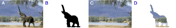
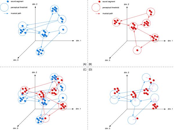
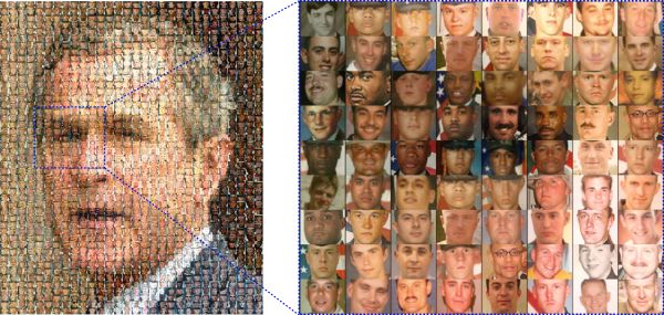
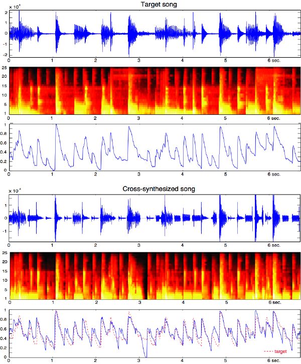
Cross-synthesis is a technique used for sound production, whereby one parameter of a synthesis model is applied in conjunction with a different parameter of another synthesis model. Physical modeling [152], linear predictive coding (LPC), or the vocoder, for instance, enable sound cross-synthesis. We extend that principle to music by synthesizing a new piece out of parameters taken from other pieces. An example application takes the music structure description of a target piece (i.e., the metadata sequence, or musical-DNA), and the actual sound content from a source piece (i.e., a database of unstructured labeled audio segments), and creates a completely new cross-synthesized piece that accommodates both characteristics (Figure 6-13). This idea was first proposed by Zils and Pachet in [181] under the name “musaicing,” in reference to the corresponding “photomosaicing” process of the visual domain (Figure 6-14).
Our implementation, however, differs from this one in the type of metadata considered, and, more importantly, the event-alignment synthesis method introduced in 6.2. Indeed, our implementation strictly preserves musical “edges,” and thus the rhythmic components of the target piece. The search is based on segment similarities—most convincing results were found using timbral and dynamic similarities. Given the inconsistent variability of pitches between two distinct pieces (often not in the same key), it was found that it is usually more meaningful to let that space of parameters be constraint-free.
Obviously, we can extend this method to larger collections of songs, increasing the chances of finding more similar segments, and therefore improving the closeness between the synthesized piece and the target piece. When the source database is small, it is usually found useful to primarily “align” source and target spaces in order to maximize the variety of segments used in the synthesized piece. This is done by normalizing both means and variances of MDS spaces before searching for the closest segments. The search procedure can be greatly accelerated after a clustering step (section 5.4.3), which dichotomizes the space in regions of interest. The hierarchical tree organization of a dendrogram is an efficient way of quickly accessing the most similar segments without searching through the whole collection. Improvements in the synthesis might include processing the “selected” segments through pitch-shifting, time-scaling, amplitude-scaling, etc., but none of these are implemented: we are more interested in the novelty of the musical artifacts generated through this process than in the closeness of the resynthesis.
|
|
|
|
Figure 6-15 shows an example of cross-synthesizing “Kickin’ Back” by Patrice Rushen with “Watermelon Man” by Herbie Hancock. The sound segments of the former are rearranged using the musical structure of the latter. The resulting new piece is “musically meaningful” in the sense that its rhythmic structure is preserved, and its timbral structure is made as close as possible to the target piece given the inherent constraints of the problem.
|
|
The final goal is to automate the creation of entirely new compositions. Our current solution is to arbitrarily combine the previous applications. Evolutionary methods could help at orienting the system; at selecting a group of sound sources, rhythmic patterns, and song structures; and at transitioning or interpolating between the parameters in such a way that the musical output reflects some of the various elements that constitute it. This part remains to be implemented. However, the system already allows us to build entire pieces with only little guidance from the user. For instance, he or she may select a set of songs that represent the source database, and a set of songs that represent the target musical structures. The system can build arbitrarily long structures, and seamlessly transition between them. It can map groups of sounds to the structures, and merge several creations via alignment and tempo curve-matching. The final outcome is a new sounding piece with apparent coherence in both the use of the sound palette, and the underlying musical structure. Yet, due to inherent constraints of our analysis-resynthesis procedure, the created music is new and different from other existing music.