“The beautiful thing about learning is that no one can take it
away from you.”
– B.B. King
Learning is acquiring knowledge or skill through study, experience, or teaching. Whether a computer system “learns” or merely “induces generalizations” is often a subject of debate. Indeed, learning from data or examples (similarity-based learning) is another way of speaking about generalization procedures and concept representations that are typically “simplistic and brittle” [119]. However, we argue that a music-listening system is not complete until it is able to improve or adapt its performance over time on tasks similar to those done previously. Therefore, this chapter introduces learning strategies that apply to the music analysis context. We believe that state-of-the-art “learning” algorithms are able to produce robust models of relatively complex systems, as long as the data (i.e., musical features) is consistent and the learning problem well posed.
Machine learning [115], a subfield of artificial intelligence [140], is concerned with the question of how to construct computer programs (i.e., agents) that automatically improve their performance at some task with experience. Learning takes place as a result of the interaction between the agent and the world, and from observation by the agent of its own decision-making processes. When learning from measured or observed data (e.g., music signals), the machine learning algorithm is also concerned with how to generalize the representation of that data, i.e., to find a regression or discrimination function that best describes the data or category. There is a wide variety of algorithms and techniques, and their description would easily fill up several volumes. There is no ideal one: results usually depend on the problem that is given, the complexity of implementation, and time of execution. Here, we recall some of the key notions and concepts of machine learning.
When dealing with music signals and extracting perceptual information, there is necessarily a fair amount of ambiguity and imprecision (noise) in the estimated data, not only due to the analysis technique, but also to the inherent fuzziness of the perceptual information. Therefore, statistics are widely used and will often play an important role in machine perception—a machine that can recognize patterns grounded on our senses. If an external teacher provides a category label or cost for each pattern (i.e., when there is specific feedback available), the learning is said to be supervised: the learning element is given the true output for particular inputs. It adapts its internal representation of a correlation function to best match the information provided by the feedback. More formally, we say that an example (or sample) is a pair (x,f(x)), where x is the input and f(x) is the output of the function applied to x. Induction is the task that, given a collection of examples of f, returns a function h (the hypothesis) that approximates f. Supervised learning can be incremental (i.e., update its old hypothesis whenever a new example arrives) or based on a representative training set of examples. One must use a large enough amount of training samples, but one must keep some for validation of the hypothesis function (typically around 30%).
In unsupervised learning or clustering, there is no explicit teacher, and the system forms “natural” clusters (groupings) of the input patterns. Different clustering algorithms may lead to different clusters, and the number of clusters can be specified ahead of time if there is some prior knowledge of the classification task. Finally, a third form of learning, reinforcement learning, specifies only if the tentative classification or decision is right or wrong, which improves (reinforces) the classifier.
For example, if our task were to classify musical instruments from listening to their sound, in a supervised context we would first train a classifier by using a large database of sound recordings for which we know the origin. In an unsupervised learning context, several clusters would be formed, hopefully representing different instruments. With reinforcement learning, a new example with a known target label is computed, and the result is used to improve the classifier.
One current way of categorizing a learning approach is differentiating whether it is generative or discriminative [77]. In generative learning, one provides domain-specific knowledge in terms of structure and parameter priors over the joint space of variables. Bayesian (belief) networks [84][87], hidden Markov models (HMM) [137], Markov random fields [177], Kalman filters [21], mixture of experts [88], mixture of multinomials, mixture of Gaussians [145], and so forth, provide a rich and flexible language for specifying this knowledge and subsequently refining it with data and observations. The final result is a probabilistic distribution that is a good generator of novel examples.
Conversely, discriminative algorithms adjust a possibly non-distributional model to data, optimizing a specific task, such as classification or prediction. Popular and successful examples include logistic regression [71], Gaussian processes [55], regularization networks [56], support vector machines (SVM) [22], and traditional artificial neural networks (ANN) [13]. This often leads to superior performance, yet compromises the flexibility of generative modeling. Jaakkola et al. recently proposed Maximum Entropy Discrimination (MED) as a framework to combine both discriminative estimation and generative probability density [75]. Finally, in [77], imitative learning is presented as “another variation on generative modeling, which also learns from examples from an observed data source. However, the distinction is that the generative model is an agent that is interacting in a much more complex surrounding external world.” The method was demonstrated to outperform (under appropriate conditions) the usual generative approach in a classification task.
Linear systems have two particularly desirable features: they are well characterized and are straightforward to model. One of the most standard ways of fitting a linear model to a given time series consists of minimizing squared errors between the data and the output of an ARMA (autoregressive moving average) model. It is quite common to approximate a nonlinear time series by locally linear models with slowly varying coefficients, as through Linear Predictive Coding (LPC) for speech transmission [135]. But the method quickly breaks down when the goal is to generalize nonlinear systems.
Music is considered a “data-rich” and “theory-poor” type of signal: unlike strong and simple models (i.e., theory-rich and data-poor), which can be expressed in a few equations and few parameters, music holds very few assumptions, and modeling anything about it must require a fair amount of generalization ability—as opposed to memorization. We are indeed interested in extracting regularities from training examples, which transfer to new examples. This is what we call prediction.
We use our predictive models for classification, where the task is to categorize the data into a finite number of predefined classes, and for nonlinear regression, where the task is to find a smooth interpolation between points, while avoiding overfitting (the problem of fitting the noise in addition to the signal). The regression corresponds to mapping a high-dimensional input data stream into a (usually) one-dimensional nonlinear output function. This one-dimensional signal may be the input data itself in the case of a signal forecasting task (section 5.2.5).
The idea of forecasting future values by using immediately preceding ones (called a time-lag vector, or tapped delay line) was first proposed by Yule [179]. It turns out that the underlying dynamics of nonlinear systems can also be understood, and their geometrical behavior inferred from observing delay vectors in a time series, where no or a priori information is available about its origin [157]. This general principle is known as state-space reconstruction [53], and inspires our predictive approach. The method has previously been applied to musical applications, e.g., for determining the predictability of driven nonlinear acoustic systems [144], for musical gesture analysis and embedding synthesis [114], and more recently for modeling musical compositions [3].
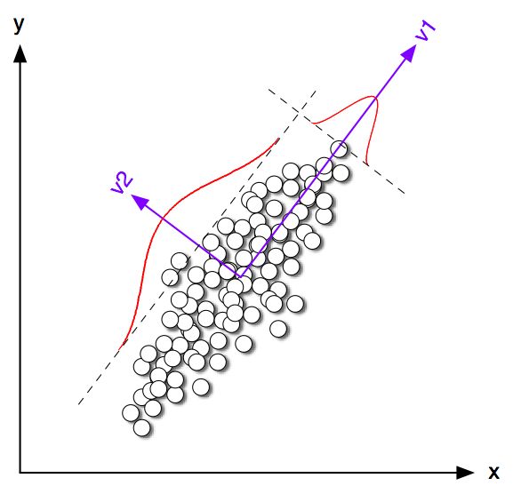
Principal component analysis (PCA) involves a mathematical procedure that transforms a number of (possibly) correlated variables into a (smaller) number of uncorrelated variables called principal components. The first principal component accounts for the greatest possible statistical variability (or entropy) in the data, and each succeeding component accounts for as much of the remaining variability as possible. Usually, PCA is used to discover or reduce the dimensionality of the data set, or to identify new meaningful underlying variables, i.e., patterns in the data. Principal components are found by extracting the eigenvectors and eigenvalues of the covariance matrix of the data, and are calculated efficiently via singular value decomposition (SVD). These eigenvectors describe an orthonormal basis that is effectively a rotation of the original cartesian basis (Figure 5-1).
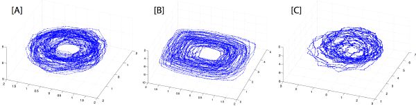
When a time-lag vector space is analyzed through PCA, the resulting first few dimensions characterize the statistically most significant underlying degrees of freedom of the dynamical system. A data set, which appears complicated when plotted as a time series, might reveal a simpler structure, represented by a manifold when plotted as a stereo plot (Figure 5-2). This apparent simpler structure provides the evidence of some embedded redundant patterns, which we seek to model through learning. Our primarily goal is to build a generative (cognitive) representation of music, rather than “resynthesize” it from a rigid and finite description. Nevertheless, a different application consists either of transforming the manifold (e.g., through rotation, scaling, distortion, etc.), and unfolding it back into a new time series; or using it as an attractor for generating new signals, governed by similar dynamics [3].
We project a high-dimensional space onto a single dimension, i.e., a correlation between the time-lag vector [xt-(d-1)τ,...,xxt-τ] and the current value xt [48]. We use machine-learning algorithms to infer the mapping, which consequently provides an insight into the underlying behavior of the system dynamics. Given an initial set of d data points, the previously taught model can exploit the embedded geometry (long-term memory) to predict a new forthcoming data point xt+1. By repeating the procedure even further through data points xt+2,...,xt+(δ-1)τ , the model forecasts the time series even farther into the future.
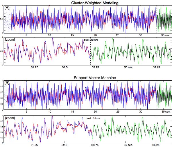
We model rhythm in this way, through both the iterative mixture of Gaussian framework (CWM) provided by Schoner [145], and a support vector machine package (SVMlight) provided by Joachims [85] (Figure 5-3). The outcome is an extremely compact “rhythm” synthesizer that learned from example, and can generate a loudness function given an initialization data set. We measure the robustness of the model by its ability to predict 1) previously trained data points; 2) new test data points; and 3) the future of the time series (both short-term and long-term accuracy). With given numbers of delays and other related parameters, better overall performances are typically found using SVM (Figure 5-3). However, a quantitative comparison between learning strategies goes beyond the scope of this thesis.
|
|
|
|
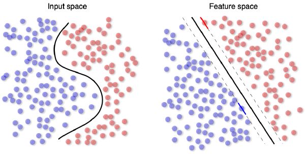
Support vector machines (SVM) [164] rely on preprocessing the data as a way to represent patterns in a high dimension—typically much higher than the original feature space. With appropriate nonlinear mapping into the new space, and through basis function, or kernel—such as Gaussian, polynomial, sigmoid function—data can always be regressed (and classified) with a hyperplane (Figure 5-4). Support vector machines differ radically from comparable approaches as SVM training always converges to a global minimum, i.e., the search corresponds to a convex quadratic programming problem, typically solved by matrix inversion. While obviously not the only machine learning solution, this is the one we choose for the following experiments.
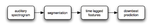
Other than modeling and forecasting one-dimensional signals, such as the loudness (rhythm) signal, we can also predict new musical information given a multidimensional input. A particularly interesting example is downbeat prediction based on surface listening, and time-lag embedded learning. The model is causal, and tempo independent: it does not require beat tracking. In fact, it could appropriately be used as a phase-locking system for the beat tracker of section 3.5, which currently runs in an open loop (i.e., without feedback control mechanism). This is left for future work.
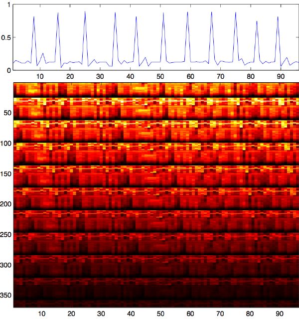
The downbeat prediction is supervised. The training is a semi-automatic task that requires little human control. If our beat tracker is accurate throughout the whole training song, and the measure length is constant, we label only one beat with an integer value pb ∈ [0,M - 1], where M is the number of beats in the measure, and where 0 is the downbeat. The system extrapolates the beat-phase labeling to the rest of the song. In general, we can label the data by tapping the downbeats along with the music in real time, and by recording their location in a text file. The system finally labels segments with a phase location: a float value ps ∈ [0,M[. The resulting segment phase signal looks like a sawtooth ranging from 0 to M. Taking the absolute value of its derivative returns our ground-truth downbeat prediction signal, as displayed in the top pane of Figure 5-5. Another good option consists of labeling tatums (section 3.4.3) rather than segments.
The listening stage, including auditory spectrogram, segmentation, and music feature labeling, is entirely unsupervised (Figure 3-19). So is the construction of the time-lag feature vector, which is built by appending an arbitrary number of preceding multidimensional feature vectors. Best results were obtained using 6 to 12 past segments, corresponding to nearly the length of a measure. We model short-term memory fading by linearly scaling down older segments, therefore increasing the weight of most recent segments (Figure 5-5).
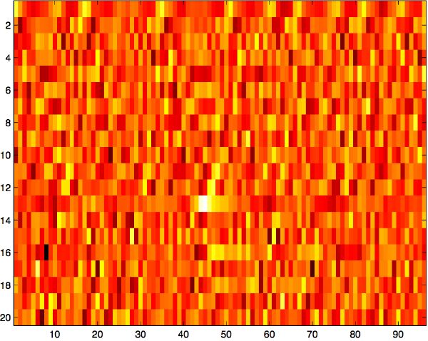
Training a support vector machine to predict the downbeat corresponds to a regression task of several dozens of feature dimensions (e.g., 9 past segments × 42 features per segments = 378 features) into one single dimension (the corresponding downbeat phase of the next segment). Several variations of this principle are also possible. For instance, an additional PCA step (section 5.2.3) allows us to reduce the space considerably while preserving most of its entropy. We arbitrarily select the first 20 eigen-dimensions (Figure 5-6), which generally accounts for about 60–80% of the total entropy while reducing the size of the feature space by an order of magnitude. It was found that results are almost equivalent, while the learning process gains in computation speed. Another approach that we have tested consists of selecting the relative features of a running self-similarity triangular matrix rather than the original absolute features, e.g., ((9 past segments)2 - 9)∕2 = 36 features. Results were found to be roughly equivalent, and also faster to compute.
|
|
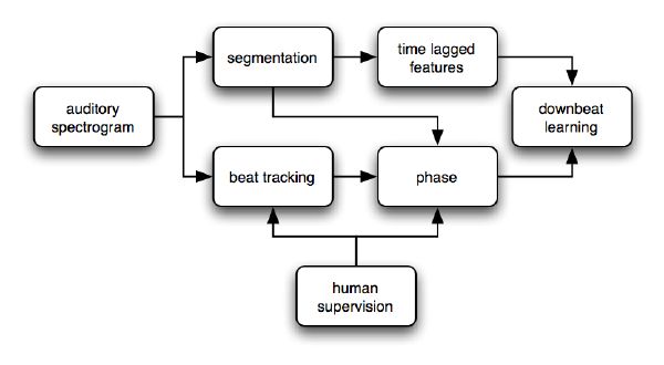
We expect that the resulting model is not only able to predict the downbeat of our training data set, but to generalize well enough to predict the downbeat of new input data—denominated test data in the following experiments. An overall schematic of the training method is depicted in Figure 5-7.
Although downbeat may often be interpreted through harmonic shift [61] or a generic “template” pattern [92], sometimes neither of these assumptions apply. This is the case of the following example.
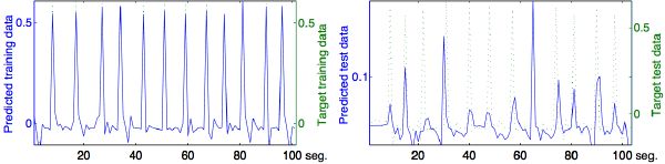
James Brown’s music is often characterized by its repetitive single chord and syncopated rhythmic pattern. The usual assumptions, as just mentioned, do not hold. There may not even be any measurable energy in the signal at the perceived downbeat. Figure 5-8 shows the results of a simple learning test with a 30-second excerpt of “I got the feelin’.” After listening and training with only 30 seconds of music, the model demonstrates good signs of learning (left pane), and is already able to predict reasonably well some of the downbeats in the next 30-second excerpt in the same piece (right pane).
|
|
Note that for these experiments: 1) no periodicity is assumed; 2) the system does not require a beat tracker and is actually tempo independent; and 3) the predictor is causal and does, in fact, predict one segment into the future, i.e., about 60–300 ms. The prediction schematic is given in Figure 5-9.
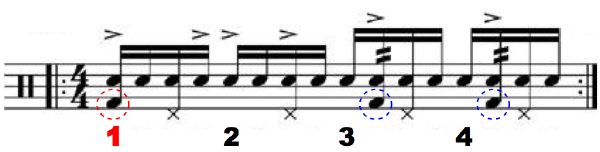
Our second experiment deals with a complex rhythm from the northeast of Brazil called “Maracatu.” One of its most basic patterns is shown in standard notation in Figure 5-10. The bass-drum sounds are circled by dotted lines. Note that two out of three are syncopated. A listening test was given to several musically trained western subjects, none of whom could find the downbeat. Our beat tracker also performed very badly, and tended to lock onto syncopated accents.
|
|
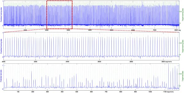
We train our model with six Maracatu pieces from the band Maracatu Estrela Brilhante. Those pieces have different tempi, and include a large number of drum sounds, singing voices, choirs, lyrics, and a variety of complex rhythmic patterns. Best results were found using an embedded 9-segment feature vector, and a Gaussian kernel for the SVM. We verify our Maracatu “expert” model both on the training data set (8100 data points), and on a new piece from the same album (1200 data points). The model performs outstandingly on the training data, and does well on the new untrained data (Figure 5-11). Total computation cost (including listening and modeling) was found to be somewhat significant at training stage (about 15 minutes on a dual-2.5 GHz Mac G5 for the equivalent of 20 minutes of music), but minimal at prediction stage (about 15 seconds for a 4-minute song).
This experiment demonstrates the workability of extracting the downbeat in arbitrarily complex musical structures, through supervised learning, and without needing the beat information. Although we applied it to extract the downbeat location, such framework should allow to learn and predict other music information, such as, beat location, time signature, key, genre, artist, etc. But this is left for future work.
Repeating sounds and patterns are widely exploited throughout music. However, although analysis and music information retrieval applications are often concerned with processing speed and music description, they typically discard the benefits of sound redundancy cancellation. Our method uses unsupervised clustering, allows for reduction of the data complexity, and enables applications such as compression [80].
Typical music retrieval applications deal with large databases of audio data. One of the major concerns of these programs is the meaningfulness of the music description, given solely an audio signal. Another concern is the efficiency of searching through a large space of information. With these considerations, some recent techniques for annotating audio include psychoacoustic preprocessing models [128], and/or a collection of frame-based (i.e., 10–20 ms) perceptual audio descriptors [70] [113]. The data is highly reduced, and the description hopefully relevant. However, although the annotation is appropriate for sound and timbre, it remains complex and inadequate for describing music.
In this section, two types of clustering algorithms are proposed: nonhierarchical and hierarchical. In nonhierarchical clustering, such as the k-means algorithm, the relationship between clusters is undetermined. Hierarchical clustering, on the other hand, repeatedly links pairs of clusters until every data object is included in the hierarchy. The goal is to group similar segments together to form clusters whose centroid or representative characterizes the group, revealing musical patterns and a certain organization of sounds in time.
K-means clustering is an algorithm used for partitioning (clustering) N data points into K disjoint subsets so as to minimize the sum-of-squares criterion:

| (5.1) |
where xn is a vector representing the nth data point and μj is the geometric centroid of the data points in Sj. The number of clusters K must be selected at onset. The data points are assigned at random to initial clusters, and a re-estimation procedure finally leads to non-optimized minima. Despite these limitations, and because of its simplicity, k-means clustering is the most popular clustering strategy. An improvement over k-means, called “Spectral Clustering,” consists roughly of a k-means method in the eigenspace [120], but it is not yet implemented.
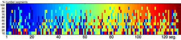
We start with the segment metadata as described in section 3.7. That MDS space being theoretically normalized and Euclidean (the geometrical distance between two points is “equivalent” to their perceptual distance), it is acceptable to use k-means for a first prototype. Perceptually similar segments fall in the same region of the space. An arbitrary small number of clusters is chosen depending on the targeted accuracy and compactness. The process is comparable to vector quantization: the smaller the number of clusters, the smaller the lexicon and the stronger the quantization. Figure 5-12 depicts the segment distribution for a short audio excerpt at various segment ratios (defined as the number of retained segments, divided by the number of original segments). Redundant segments get naturally clustered, and can be coded only once. The resynthesis for that excerpt, with 30% of the original segments, is shown in Figure 5-14.
|
|
One of the main drawbacks of using k-means clustering is that we may not know ahead of time how many clusters we want, or how many of them would ideally describe the perceptual music redundancy. The algorithm does not adapt to the type of data. It makes sense to consider a hierarchical description of segments organized in clusters that have subclusters that have subsubclusters, and so on.
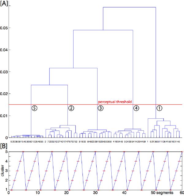
Agglomerative hierarchical clustering is a bottom-up procedure that begins with each object as a separate group. These groups are successively combined based on similarity until there is only one group remaining, or a specified termination condition is satisfied. For n objects, n - 1 mergings are done. Agglomerative hierarchical methods produce dendrograms (Figure 5-13). These show hierarchical relations between objects in form of a tree.
|
|
We can start from a similarity matrix as described in section 4.2.4. We order segment pairs by forming clusters hierarchically, starting from the most similar pairs. At each particular stage the method joins together the two clusters that are the closest from each other (most similar). Differences between methods arise because of the different ways of defining distance (or similarity) between clusters. The most basic agglomerative model is single linkage, also called nearest neighbor. In single linkage, an object is linked to a cluster if at least one object in the cluster is the closest. One defect of this distance measure is the creation of unexpected elongated clusters, called the “chaining effect.” On the other hand, in complete linkage, two clusters fuse depending on the most distant pair of objects among them. In other words, an object joins a cluster when its similarity to all the elements in that cluster is equal or higher to the considered level. Other methods include average linkage clustering, average group, and Ward’s linkage [42].
The main advantages of hierarchical clustering are 1) we can take advantage of our already computed perceptual similarity matrices; 2) the method adapts its number of clusters automatically to the redundancy of the music; and 3) we can choose the level of resolution by defining a similarity threshold. When that threshold is high (fewer clusters), the method leads to rough quantizations of the musical description (Figure 5-13). When it is low enough (more clusters) so that it barely represents the just-noticeable difference between segments (a perceptual threshold), the method allows for reduction of the complexity of the description without altering its perception: redundant segments get clustered, and can be coded only once. This particular evidence leads to a compression application.
Compression is the process by which data is reduced into a form that minimizes the space required to store or transmit it. While modern lossy audio coders efficiently exploit the limited perception capacities of human hearing in the frequency domain [17], they do not take into account the perceptual redundancy of sounds in the time domain. We believe that by canceling such redundancy, we can reach further compression rates. In our demonstration, the segment ratio indeed highly correlates with the compression rate that is gained over traditional audio coders.
|
|
Perceptual clustering allows us to reduce the audio material to the most perceptually relevant segments, by retaining only one representative (near centroid) segment per cluster. These segments can be stored along with a list of indexes and locations. Resynthesis of the audio consists of juxtaposing the audio segments from the list at their corresponding locations (Figure 5-14). Note that no cross-fading between segments or interpolations are used at resynthesis.
If the threshold is chosen too high, too few clusters may result in musical distortions at resynthesis, i.e., the sound quality is fully maintained, but the musical “syntax” may audibly shift from its original form. The ideal threshold is theoretically a constant value across songs, which could be defined through empirical listening test with human subjects and is currently set by hand. The clustering algorithm relies on our matrix of segment similarities as introduced in 4.4. Using the agglomerative clustering strategy with additional supervised feedback, we can optimize the distance-measure parameters of the dynamic programming algorithm (i.e., parameter h in Figure 4-4, and edit cost as in section 4.3) to minimize the just-noticeable threshold, and equalize the effect of the algorithm across large varieties of sounds.
Reducing audio information beyond current state-of-the-art perceptual codecs by structure analysis of its musical content is arguably a bad idea. Purists would certainly disagree with the benefit of cutting some of the original material altogether, especially if the music is entirely performed. There are obviously great risks for music distortion, and the method applies naturally better to certain genres, including electronic music, pop, or rock, where repetition is an inherent part of its qualities. Formal experiments could certainly be done for measuring the entropy of a given piece and compressibility across sub-categories.
We believe that, with a real adaptive strategy and an appropriate perceptually grounded error estimation, the principle has great potential, primarily for devices such as cell phones, and PDAs, where bit rate and memory space matter more than sound quality. At the moment, segments are compared and concatenated as raw material. There is no attempt to transform the audio itself. However, a much more refined system would estimate similarities independently of certain perceptual criteria, such as loudness, duration, aspects of equalization or filtering, and possibly pitch. Resynthesis would consist of transforming parametrically the retained segment (e.g., amplifying, equalizing, time-stretching, pitch-shifting, etc.) in order to match its target more closely. This could greatly improve the musical quality, increase the compression rate, while refining the description.
Perceptual coders have already provided us with a valuable strategy for estimating the perceptually relevant audio surface (by discarding what we cannot hear). Describing musical structures at the core of the codec is an attractive concept that may have great significance for many higher-level information retrieval applications, including song similarity, genre classification, rhythm analysis, transcription tasks, etc.