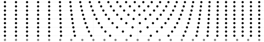
Early American Experimental Music

American composer Charles Ives (1874-1954) wrote many experimental pieces where he would selectively disregard certain ‘rules’ of music theory, and explore the sonic results. In an essay on his experimental music, Ives asked this question:

If you can play a tune in one key, why can’t a feller, if he feels like, play one in two keys?

Ives’ early polytonal experiments include pieces with a melody in one musical key and accompaniment in another key, and pieces with separate voices, each in separate keys. These experimental pieces were not published or performed until long after he wrote them, but Ives’ ideas did appear in his less systematic compositions. More importantly his ideas influenced a generation of younger composers.

Among these younger composers was Henry Cowell (1897-1965), who in 1930 published New Musical Resources, a collection of largely unexplored musical ideas. The book extends the notion of multiple simultaneous musical keys polytonal music to multiple simultaneous tempos, polytempic music.

Can we make music with multiple simultaneous tempos? Certainly. But Cowell took the idea a step further. Assume we have multiple simultaneous tempos and these tempos are accelerating or decelerating relative to each other. In New Musical Resources, Cowell called this practice sliding tempo, and he noted that this would not be easy to do. In 1930, he writes:

For practical purposes, care would have to be exercised in the use of sliding tempo, in order to control the relation between tones in a sliding part with those in another part being played at the same time: a composer would have to know in other words, what tones in a part with rising tempo would be struck simultaneously with other tones in a part of, say, fixed tempo, and this from considerations of harmony. There would usually be no absolute coincidence, but the tones which would be struck at approximately the same time could be calculated.

Phase Music

Can we calculate the times of coincidence like Cowell suggests? How? Can a musician even perform polytempic music with tempo accelerations or decelerations? Over the course of the 20th century, musicians explored this idea in what is now called phase music (wikipedia). One early example is Piano Phase (1967) by Steve Reich (wikipedia, vimeo).

Through experimentation, Steve Reich found that if the music is reasonably simple, two performers can make synchronized tempo adjustments relative to each other well enough to yield compelling results. In Piano Phase two pianos both play the same repeating 12 note musical pattern. One musician plays at a slightly faster rate than the other. It is possible for a musician to play this, but there is a limit to complexity of the patterns that a musician can play and a limit to the number of simultaneous changing tempi a musician can comprehend. Piano Phase approaches the limit of what a musician can perform. Can we not use electronic sequencers or digital audio tools to synthesize complex phase music with many simultaneous tempic transitions?

Most phase music (including Piano Phase) layers identical copies of musical content playing at slightly different speeds. The layers begin in-phase with with each other, and gradually drift out of phase. Reich’s Piano Phase is no exception. As the layers drift out of phase, our listening attention is drawn to variations caused by shifting phase relationships between the layers. In the example below, the two layers start out playing together at 90 beats-per-minute (BPM), at \(t=0\) the top layer abruptly starts playing at 100 BPM.

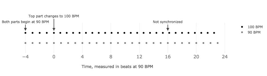
If we wait long enough, eventually the layers will re-align, and and the whole pattern will start from the beginning again. But what if we want to control exactly when the layers re-synchronize? Can we specify precisely both the time and the phase of sync points without abrupt changes in tempo? How can we sequence patterns like the one below exactly? This is the central question of Tempic Integrations.

Tempic Integrations

If we want to specify the exact number of beats that elapse between the beginning of a tempo acceleration and the end point of the acceleration, and we want to hear this precisely we need a mathematical model for shaping our tempo acceleration curves. The goal is to compose and audition music where:

• Swarms of an arbitrary number of simultaneous tempi coexist.
• Each individual player within the swarm can continuously accelerate or decelerate individually, but also as a member of a cohesive whole.
• Each musical line can converge and diverge at explicit points. At each point of convergence the phase of the meter within the tempo can be set.

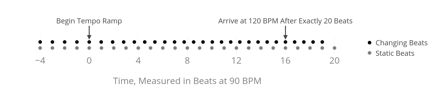
We start by defining a single tempo transition. Consider the following example from the image above:

• Assume we have 2 snare drum players. Both begin playing the same beat at 90 BPM in common time.
• One performer gradually accelerates relative to the other. We want to define a continuous tempo curve such that one drummer accelerates to 120 BPM.
• So far, we can easily accomplish this with a simple linear tempo acceleration. However, we want the tempo transition to complete exactly when both drummers are on a down-beat, so the combined effect is a 3 over 4 rhythmic pattern. Linear acceleration results in the transition completing at an arbitrary phase.
• We want the accelerating drummer to reach the new tempo after exactly 20 beats.
• We also want the acceleration to complete in exactly 16 beats of the original tempo, so that the drummer playing a constant tempo and the accelerating drummer are playing together.

We are interested in both the number of beats elapsed in the static tempo and in the changing tempo, as well as the absolute tempo. If we think of the number of beats elapsed as our position, and the tempo as our rate, we see how this resembles a physics problem. If we have a function that describes our tempo (or rate), we can integrate that function, and the result will tell us our number of beats elapsed (or position). Given the above considerations, our tempo curve is defined in terms of 5 constants:

• Time \(t_0=0\), when the tempo transition begins
• A known time, \(t_1\), when the tempo transition ends
• A known starting tempo: \(\dot{x}_0\)
• A known finishing tempo: \(\dot{x}_1\)
• The number of beats elapsed in the changing tempo between \(t_0\) and \(t_1\): \(x_1\)

The tension of the tempo curve determines how many beats elapse during the transition period. The curve is well-defined for some starting acceleration \(a_0\) and finishing acceleration \(a_1\), so we define the curve in terms of linear acceleration. Using Newtonian notation we can describe our tempo acceleration as:

\[\begin{equation} \ddot{x}_1 = a_0 + a_1t_1 \end{equation}\]

Integrating linear acceleration (above) yields a quadratic velocity curve (below). The velocity curve describes the tempo (in beats per minute) with respect to time.

\[\begin{equation} \dot{x}_1 = \dot{x}_0 + a_0t_1 + \frac{a_1t_1^2}{2} \end{equation}\]

Integrating velocity (above) gives us a function describing position (the number of beats elapsed with respect to time, below).

\[\begin{equation} x_1 = x_0 + \dot{x}_0t_1 + \frac{a_0t_1^2}{2} + \frac{a_1t_1^3}{6} \end{equation}\]

With equations for \(\dot{x}_1\) and \(x_1\), we can solve for our two unknowns, \(a_0\) and \(a_1\). First we solve both equations for \(a_1\):

\[\begin{equation} a_1 = \frac{-2}{t_1^2}(\dot{x}_0-\dot{x}_1 + a_0t_1) = \frac{-6}{t_1^3}(\dot{x}_0t_1-x_1 + \frac{a_0t_1^2}{2}) \end{equation}\]

Assuming \(t_1 \neq 0\), we solve this system of equations for \(a_0\):

\[\begin{equation} a_0=\frac{6x_1-2t_1(\dot{x}_1+2\dot{x}_0)}{t_1^2} \end{equation}\]

Evaluating for \(a_0\) with our constants gives us our starting acceleration. Once we have \(a_0\) we can solve our velocity equation to find the value of \(a_1\). Plugging \(a_1\) and \(a_0\) into the velocity equation will give us velocity curve that produces a continuous BPM curve over the course of the tempo transition.

Note: We must specify the same time units for input variables like \(t_1\) and \(\dot{x}_1\). I prefer minutes for \(t_1\) and beats per minute for \(\dot{x}_1\) over seconds and beats per second.